WCOJ - Graph-Join correspondence

An introduction and motivation for Worst Case Optimal Joins

Consider the TPC-H query 5 (Local Supplier Volume) and just focus on the join part of the query. TPC-H is standardised benchmark with very common business queries on a synthetic dataset.

 SELECT
    n_name,
    SUM(l_extendedprice * (1 - l_discount)) AS revenue
FROM
    customer
    JOIN orders ON c_custkey = o_custkey
    JOIN lineitem ON l_orderkey = o_orderkey
    JOIN supplier ON l_suppkey = s_suppkey AND c_nationkey = s_nationkey
    JOIN nation ON s_nationkey = n_nationkey
    JOIN region ON n_regionkey = r_regionkey
WHERE
    r_name = 'ASIA'
    AND o_orderdate >= DATE '1994-01-01'
    AND o_orderdate < DATE '1994-01-01' + INTERVAL '1' YEAR
GROUP BY
    n_name
ORDER BY
    revenue DESC; 

If we create a graph for this query where nodes represent join variables (in SQL these are just join conditions as the notion of a join variable does not really exist in SQL) and where edges represent relations (tables), we get the following diagram. Notice that this is a hypergraph as relations might participate in more than 2 joins.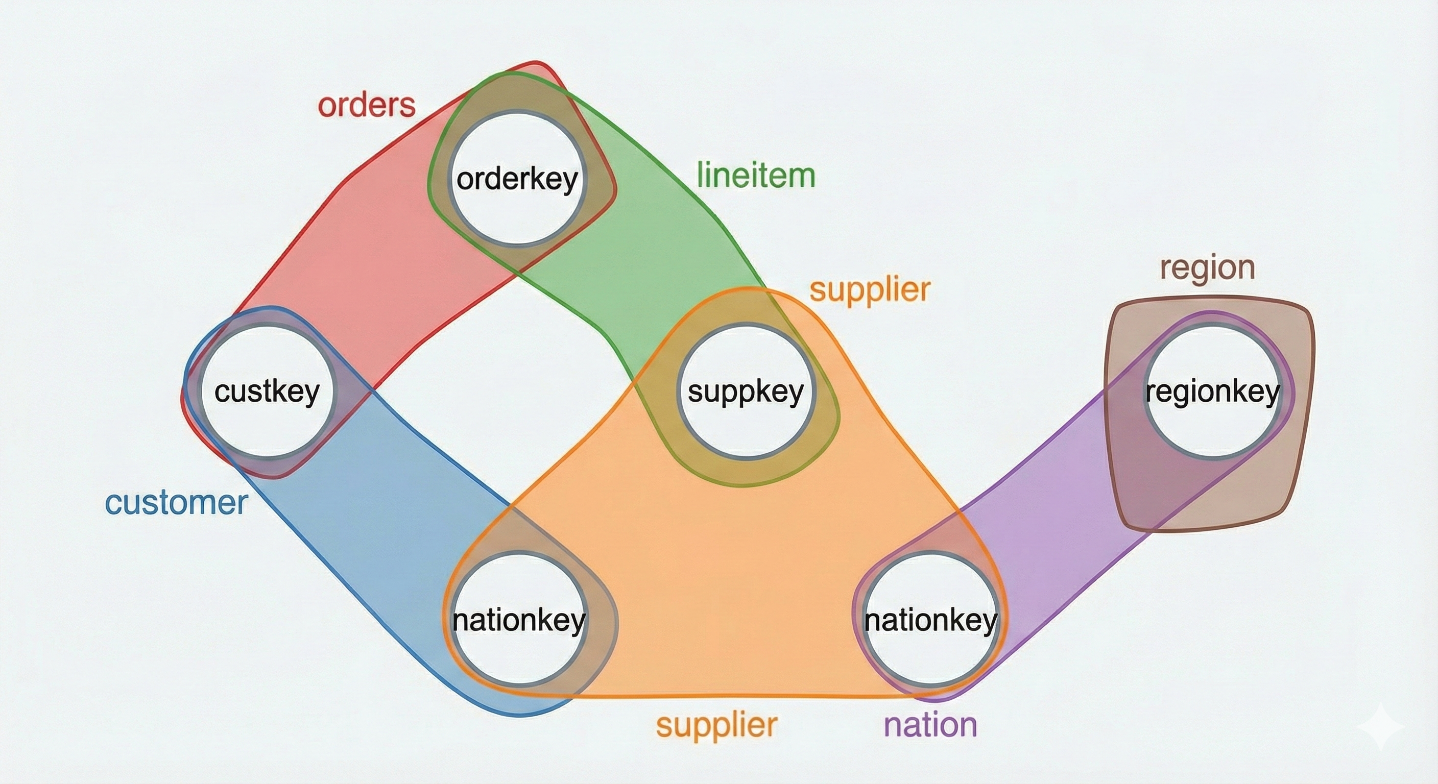 There is a direct correspondence between graphs and joins. There are even whole database vendors who have made their data model graphs. Albeit in most cases the underlying model is for standard graphs (binary edges). You can of course also go the other way around and model graphs in the relational model.

CREATE TABLE g(f INT, t INT);

Finding all triangles in a graph can then be modelled as

SELECT
    g1.f AS a, g1.t AS b, g2.t AS c
FROM
    g AS g1, g AS g2, g AS g3
WHERE
    g1.t = g2.f AND g2.t = g3.t AND g1.f = g3.f;

The main difference between this query and former one is that we are doing self joins. The similarity is that we are looking for a certain kind of pattern in our data. A triangle in the latter case and a more involved pattern in the TPC-H case.

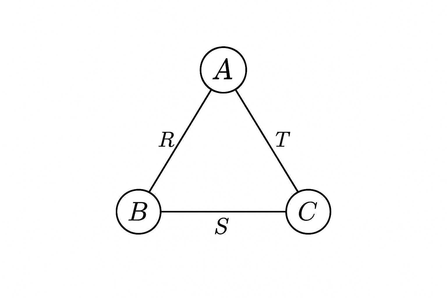
Writing the triangle in terms of three different relations you get

and the corresponding hypergraph (which is just a standard graph in this case)

I also want to have a look at the triangle query in EDN Datalog . It looks in my opinion a lot cleaner and anticipates some of the explanations coming in later posts. The systems of the variant of Datalog I am interested in store data as EAV (Entity - Attribute - Value) triples (also sometimes called Subject - Predicate - Object in other contexts) where facts are stored as entities with an attribute name and a value. So for example

[1 :name "Ada Lovelace"]

would mean an entity with id 1 (presumably a person), where the name is "Ada Lovelace". The triangle query in this model would look as follows. Entities are just nodes pointing at other nodes.

{:find [?a ?b ?c]
 :where [[?a :g/to ?b]
         [?a :g/to ?c]
         [?b :g/to ?c]]}

The symbols starting with ? are variables and are implicitly joined (equi-join) with all other occurrences of the variable. The :where section of a query limits the combinations of possible results by pattern matching the clauses against the EAV index of the database. In this case 3 triple clauses that specify the edges. You can think of the :find part as the projection of the query. By default such databases have different permutations of the EAV index (most have at leastEAV, AEV and AVE as indices). These indices will become important in later posts. In this model the edges of the graph have an implicit direction, but we can assume an edge is only present if ?from < ?to for all clauses matching [?from :g/to ?to].

Once the relationship between graphs and joins is established, one can ask all kinds of questions on graphs and wonder what it means for joins. Let’s take some common graph problems and see what that corresponds to in terms of joins (with the hypergraph definition from above):

• Vertex cover - A set of variables (join conditions) that touch every relation of the query. Correspondingly a minimum vertex cover is the smallest set (in size) of variables touching every relation.
• Independent set - A set of variables that pairwise don’t share a relation.
• Clique- It’s just the dual of the independent set, so a set of variables that pairwise share a relation.
• Edge Cover - A set of relations so that every variable (join) is covered by some relation. I want to formalize the edge cover a bit more as it will become important further down. Let $n$ be the number of relations. Let $H_Q$ be the hypergraph of a query as defined above. We let $E_Q$ be the (hyper) edges of the query graph. Informally we have $E_Q = \bigcup_{i \in [n]} R_i$ (relations are just edges). An edge cover of of $H_Q$ is then a subset of $E_Q$ so that every variable is covered. For the triangle query any two edges suffice. For the TPC-H example from above orders, supplier and region would be an edge cover.

This list could go on and on. I think the main takeaway here is that results in graph theory might have immediate implications for joins and it’s likely good to switch back and forth between these two representations when working on a join problem.

In the following we assume that every row in a table / relation is unique. We are also only taking about equi-joins. This is not the case for SQL but will help us to keep things simple.

First let’s establish some bounds for simple binary joins ¹ and then extend these to multijoins. I think the most obvious bound for a join is

You can have no more rows than the size of the tables multiplied. For this bound to be met every row would need to join with every other row. But as we are talking about equi-joins (or natural joins), a join can only reduce the size of a table so we also have the bound

If we extend this to multiple relations (let’s say $k$) that all participate in a join on variable $A$ , we obtain

An edge cover of the hypergraph of a query let’s us obtain a bound on the output size of the whole query. Let’s unpack this a bit. For every variable participating in the query there is a set of relations (edges) that cover this variable. As the formula just above shows, any size of a participating relation is an upper bound for that particular join variable.

An edge cover of the query graph is a set of relations that cover every participating variable. This means the product of sizes of these relations is an upper bound on the output size of the whole query. Writing this down more formally. Let $x_i$ be 1 if $R_i \in E_Q$ and 0 otherwise. This let’s us then conveniently write $|R_i|^{x_i}$ to get the size of the relation depending on whether $R_i$ is participating in the edge cover or not. Putting all this notation into one formula we are getting for a given edge cover $E_Q$

This is just $N^2$ for the triangle query as you only need to pick two edges to get an edge cover. For the TPC-H query above, an upper bound would be $|orders||supplier||region|$.

If you think just about the triangle query case you can also find this bound without any machinery. Once you have chosen a 2-path in a graph ($O(N^2)$), the number of results can only go down as the closing edge of the triangle only restricts results.

This finally brings us to the graph-theoretic result that initially sparked the worst-case optimal join gold rush ². I won’t go into the details of how this result is obtained as that is way beyond the scope of this post. The result shows that you can relax the integer constraints in $\text{(AGM)}$ of the edge cover from

to

and still obtain a valid bound on the output size of the query $Q$. Let $E_{Q(A)}$ be the set of hyperedges that participate in the join on variable $A$. The relaxed version would have the constraint that

and also for all other join variables participating in the query. The relaxation from the binary decision of taking an edge or not into the edge cover to partially taking an edge is called a fractional edge cover. The bound you obtain via the relaxed edge cover is also often abbreviated as AGM bound.

We can get a simpler formula by making some assumptions. Let $Q$ be a query over relations $R_1, R_2, …, R_m$ with $|R_i| \approx N$ the output size of $Q$ can be bound by

where $\rho$ is the size of the minimum edge cover and $\rho^*$ is the size of the minimum fractional edge cover. This simply plugging the assumption $|R_i| \approx N$ into $\text{(AGM)}$.

Coming back to the triangle query

the bound then simplifies to

by assigning every edge of the triangle query hypergraph a weight of $1/2$. This assignment satisfies the relaxed constraints of the fractional edge cover. This actually means any graph can have at most $N^{3/2}$ triangles!!!

For joins it means that any binary join strategy for the triangle query will potentially produce $O(N^2)$ intermediate result rows but the AGM bound proves there can never be more than $O(N^{3/2})$ result rows. The whole idea of Worst Case Optimal Join (WCOJ henceforth) is to join the relations in such a manner that we don’t go over the worst-case bound (the specific bound depends of course on the query and the size of the involved relations).

A WCOJ algorithm guarantees that you are not doing worse then the most degenerate case. As an example, there are graphs that have $O(N^{3/2})$ triangles and in that case it assures that no larger than $O(N^{3/2})$ intermediate result sets are created. For any graph having $o(N^{3/2})$ triangles, a WCOJ algorithm does not guarantee you to run in $o(N^{3/2})$. This is the worst part of WCOJ. Also keep in mind that variable ordering still plays an important role in pruning early.

It’s unlikely that you search for arbitrary graph patterns in a relational database, but in theory you could and in graph databases it is also way more likely. The TPC-H example shows there are queries that contain cycles and where binary join strategies might exhibit degenerate behaviour. Also keep in mind that WCOJ is still in its infancy compared to binary joins. So even if a WCOJ might guarantee you certain properties, in practice it might be that binary joins fare very well as they have been optimized for decades. ³

In the next post we will look at concrete WCOJ algorithm.