WCOJ - DBSP, ZSets and Datalog

Tying together DBSP and updates in a Datalog engine in preparation for a WCOJ for DBSP

The folks from Feldera have written some good blog posts on Z-sets and their implementation. Reading them will make what follows a lot easier (but it’s hopefully not a requirement). I am also going to use some notation from their DBSP paper ¹.

In previous posts (1, 2, 3) we saw the implementation of a WCOJ algorithm called GenericJoin and how parts of the EDN Datalog query language could be implemented via concrete instantiations of the GenericJoin PrefixExtender interface. In this post we are going to do a detour to DBSP. DBSP is an incremental view maintenance framework. Given a database $DB$ and a query $Q$, the incremental view maintenance (IVM) problem concerns itself with calculating the changes to the query $\Delta Q$ by only processing the changes (inserts, updates and deletes) $\Delta DB$ to the database. DBSP gives a framework to incrementalize all of relational algebra and stratified datalog. Datomic-style Datalog engines are essentially stratified Datalog, as negation clauses are only evaluated when all variables in the negated part are bound. This means given a SQL or Datalog query $Q$, DBSP gives a method to calculate updates to the query efficiently.

Efficiency

So, given database $DB$ and some changes $\Delta DB$ (I just think of this as a transaction) to the database. An incremental version of a query outputs the changes to the query through transaction history. Most of the time I will just be using query to mean the incremental version of the query (also sometimes called a streaming query). A standard database query works on the database snapshots. Streaming queries work on a stream of changes/transaction to the database. From context it should be clear of which query type I am writing about. In the DBSP paper the standard and streaming query are distinguished by $S$ and $S^\Delta$, but I will just drop the superscript for now. A simple example for the streaming version of a query would be, given the query

{:find [person name]
 :where [person :name name]}

and the transaction

[[:db/add 1 :name "Ada Lovelace"]]

one would obtain the result (assuming Ada Lovelace is not yet part of the db)

#{[[1 "Ada Lovelace"] 1]}

The entity id 1 for a person with the name “Ada Lovelace” were added to the database with a multiplicity of 1.

By efficient I mean that for most cases these changes can be calculated without reevaluating the whole query from scratch. The assumption always being that $|\Delta DB| \ll |DB|$. For many linear operators like filter, map and project this is $O(|\Delta DB|)$.
As the following example shows this bound doesn’t hold in the triangle query case (for joins). A single edge deletion can trigger a $O(n)$ output changes.

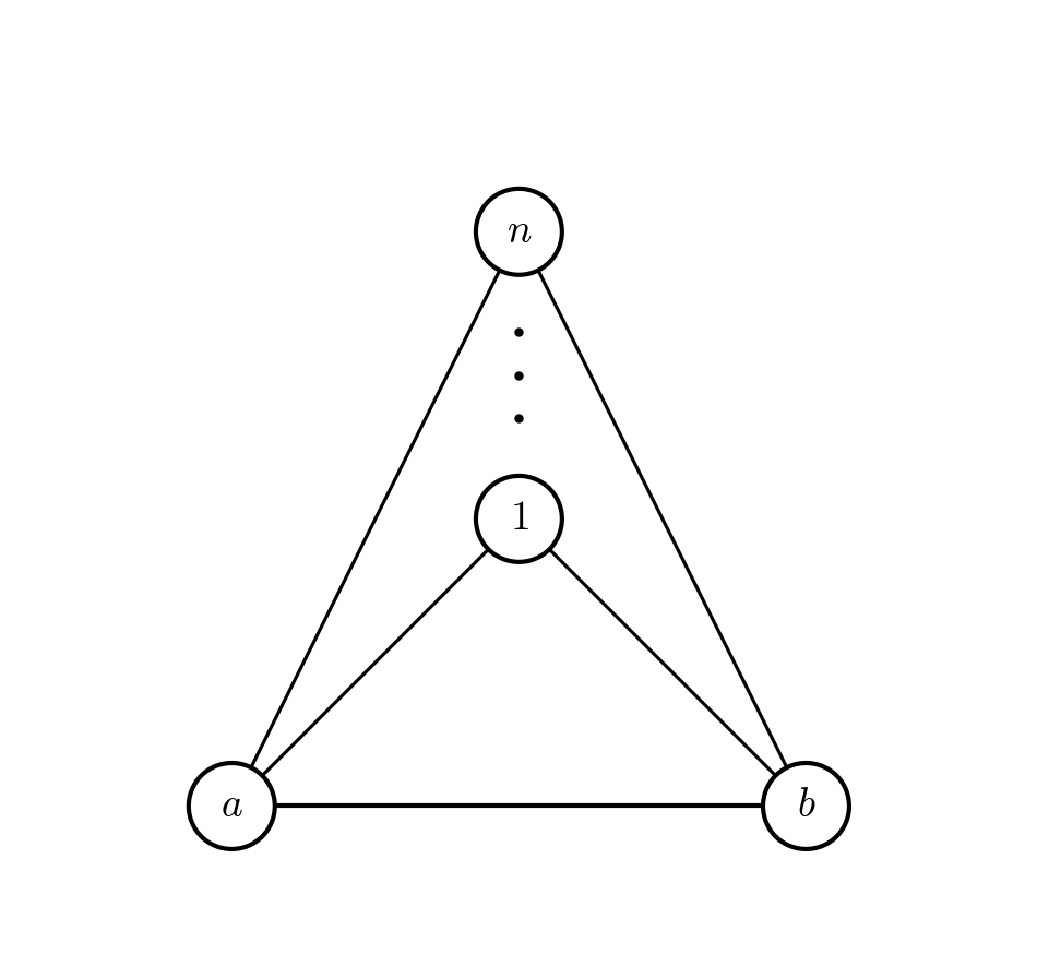The edge deletion of $(a,b)$ removes all triangles from the graph. We can do even worse (argh !). Consider the following graph 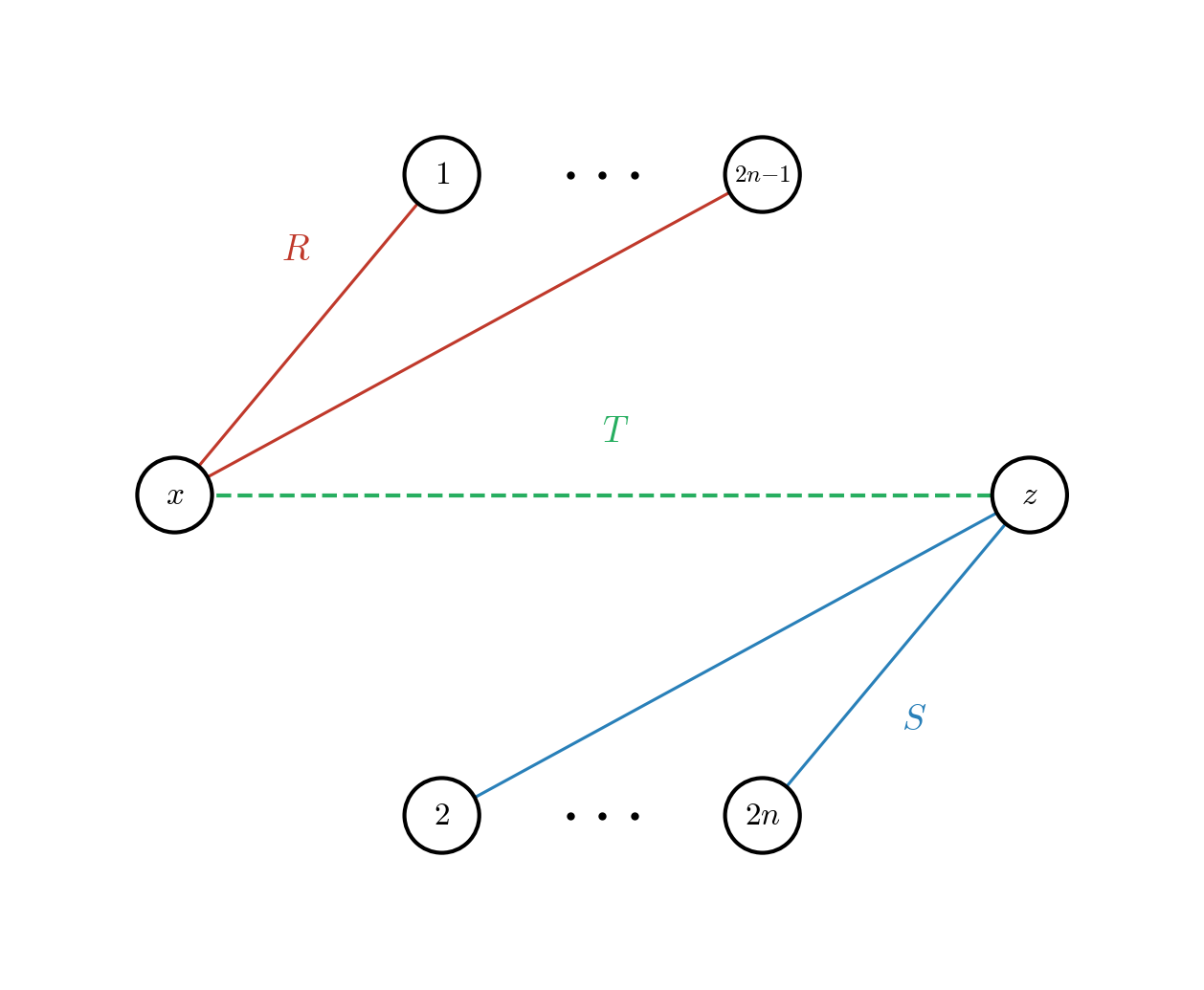from the beloved triangle query perspective.

with the setup of

and the variable join order of $(x,y,z)$. When inserting the tuple $T(1,1)$ no triangles get created, so there are no output changes, but we still need to intersect $R$ and $S$ on $y$. This intersection is empty, but the intersection will always take $O(n)$ even with a WCOJ algorithm.

The important part is that joins in DBSP are still more efficient then doing a naive reevaluation of the join, mainly $O(|DB| × |\Delta DB|)$ instead of $O(|DB|^2)$.

Similarly for recursive queries. Let’s say you calculate the transitive closure of a graph (using [from :g/to to] triples as in our first post).

 '{:find [?a ?b]
   :where [(reachable ?a ?b)] 
   :rules [[(reachable ?a ?b)
	        [?a :g/to ?b]]
           [(reachable ?a ?b)
            [?a :g/to ?c]
            (reachable ?c ?b)]]]})

The calculation involved in finding the transitive closure is finding a fixpoint where reachable states don’t grow anymore. Any addition or retraction of an edge could trigger the recalculation of that fixpoint and potentially has consequences that propagate to all output tuples, meaning the work is also no longer bound by $O(|\Delta DB |)$, but rather some polynomial in $|DB|$ which is of course not efficient in the strictest sense. DBSP will in most cases still perform better than an naive version ($O(|DB| |\Delta DB|)$ vs $O(|DB| ^{2})$ for the transitive closure).

In what follows I will use EDN notation for maps. For example

;; simple map
{key1 value1, key2 value2}
;; nested map
{key1 {nested-key1 value1, nested-key2 value2}, ...}

Z-Sets

Z-Sets are the fundamental building block of DBSP so I want to give some intuition of how they work. Z-Sets are a generalisation of sets and bags. Every element in the set has a multiplicity and the multiplicity might be negative. This allows to represent 2 kinds of data in a database system:

• The state of a relation/table/index
• The changes to a relation by a transaction A transaction produces changes in a database system. For additive changes the weights in the Z-set representation are positive and for deletions they are negative.

Z-Sets are not maps per se, as they are considered sets, but fundamentally they are backed by maps (at least in a simple implementation, see implementing Z-sets for an example), so I am going to abuse the map notation from above a bit and write Z-sets as maps.

{"Alice" 1 "Bob" -3}

This map would mean that element Alice has a multiplicity of 1 and that Bob has a multiplicity of -3. Z-sets have the nice property that they form an abelian group (don’t worry if you don’t know what that means). You can add and subtract Z-sets like normal sets and they behave nicely. For example

{"Alice" 1, "Bob" -3}
+
{"Eve" -1 "Bob" 2}
;; =>
{"Alice" 1, "Bob" -1, "Eve" -1}

This operation can be implemented efficiently on Z-sets. You can also define the negation of a Z-set which negates all weights. The empty Z-set behaves like 0 for addition and subtraction. Scalar multiplication of a Z-set multiplies all weights by the scalar. All of this means Z-sets have nice mathematical properties.

An equi-join of two Z-sets is multiplying the weights of two matching keys (non matching keys can be thought of as having a counter-part of multiplicity 0).

{"Alice" 1, "Bob" -3}
join
{"Alice" -1, "Eve" -1 "Bob" 2}
;; =>
{"Alice" -1, "Bob" -6} 

Indexed Z-Sets

Indexed Z-sets extend Z-sets by adding structure that enables efficient lookups and grouping. An indexed Z-set is essentially a map from keys to Z-sets of values. You can think of it as grouping elements by some key, where each key maps to a Z-set of associated values with their multiplicities.

{:accounting {"Alice" 1, "Bob" 2}
 :engineering {"Eve" 1, "Charlie" -1}}

This indexed Z-set groups people by department. The outer structure is the index (department), and each value is itself a Z-set of people with their multiplicities. Indexed Z-sets still form an abelian group. You add them by merging keys and adding the inner Z-sets pointwise:

{:accounting {"Alice" 1}, :engineering {"Eve" 2}}
+
{:accounting {"Bob" 1}, :engineering {"Eve" -1}}
;; =>
{:accounting {"Alice" 1, "Bob" 1}, :engineering {"Eve" 1}}

Aggregation over indexed Z-sets works by applying a function to each inner Z-set. For example, summing the multiplicities within each group:

{:accounting {"Alice" 1, "Bob" 2}, :engineering {"Eve" 1}}
;; aggregate (sum multiplicities) =>
{:accounting 3, :engineering 1}

Linear aggregates like sum and count incrementalize cleanly. Non-linear aggregates like min, max, and distinct count require more sophisticated treatment (often involving auxiliary state) to maintain incrementally.

Updates to the EAV, AEV and VAE indices

If you have not been following along AEV and VAE are permutations of the primary entity-attribute-value (EAV) index, which is the backbone of the toy-Datalog engine² we have been considering along these posts. As we have seen above, any deletion or addition in Datalog can be modelled in terms of Z-Sets. So for example the transaction

[[:db/add 1 :name "Ada Lovelace"]
 [:db/rectract 2 :name "Alan Turing"]]

can be modelled as a Z-Set of the form

{[1 :name "Ada Lovelace"] 1
 [2 :name "Alan Turing"]  -1}

We can also model these updates as nested indexed Z-Sets. So instead of having the full row as the key of our Z-Set we have the entity id on the first level, the attribute on the second and the values on the final level. For the transaction above and the EAV index this results in the following nested indexed Z-set.

{1 {:name {"Ada Lovelace" 1}}
 2 {:name {"Alan Turing" -1}}}

For the AEV and VAE indices you get similar indexed Z-sets with the entity, attribute and value permutated accordingly. I am not sure if indexed Z-sets were supposed to be used in DBSP in this manner. One could also imagine a standard Z-set but backed by some kind of opaque trie underneath. The important part is that this representation allows us to efficiently look up changes by a prefix.

Efficient multi-joins in DBSP

DBSP defines its operators over streams, an infinite sequences of Z-sets indexed by time. However, at each tick the actual computation works with Z-sets: the current deltas arriving and the accumulated state from previous ticks (not every operator needs the previous state, but some do). In what follows, I’ll write $A^\Delta$ for the delta arriving at the current tick and $A^{-1}$ for the accumulated state just before that current delta is applied. Both are Z-sets. The formulas hold at every tick. I’ll leave the time index implicit. I am also using the notation $R^A$ to denote relation $R$ restricted to variable $A$. This is to disambiguate something like $R_1^A \bowtie R_2^A$ from $R_1 \bowtie R_2$ when $R_1$ and $R_2$ share more than one join variable.

With this notation, the incremental join is given by the bilinear formula:

The output delta is computed from three terms: the join of the two input deltas, and two “cross terms” joining each delta with the other input’s previous state. Expanding out $(A \bowtie B \bowtie C)^\Delta$ already gives you 7 terms. So this won’t scale well if you do multi-joins naively. Let’s say we want to compute

using the binary join forumla above we can obtain the following recursive formula to calculate the full result.

with $\Delta_{1..i}$ being the result for the first $i$ deltas. You can obtain this formula by applying the standard join formula on $\Delta_{1..{i-1}}$ and $R_i^A$. Going from $\Delta_{1..{i-1}}$ to $\Delta_{1..i}$ means joining the previous delta accumulation $\Delta_{1..i-1}$ with the delta under consideration $\Delta R_i^A$ , the previous accumulation with the delayed relations $(R_i^A)^{-1}$ and the delta under consideration with all the delayed relations indexed by less than $i$. Notice that for $i=2$ this is the standard DBSP join formula. The left side of all three terms of the formula is a delta, meaning the joins at each iteration are bounded by $O(|\Delta DB||DB|)$, hence the the whole process is bounded by $O(|\Delta DB||DB|)$ for fixed query. We will be use this join formula when implementing the variable join (similar to the GenericSingleJoin from the second post in the series) by level for a GenericJoin-like implementation in DBSP.

Full database history in support of DBSP

In DBSP you (sometimes) need to store state history for the DBSP circuits to work correctly. Looking at the join operator formula from above once more:

$A^{-1}$ is the full relation just before applying the current delta. One insight I had while writing this post was that databases that have full history give you the previous state essentially for free. This assumes $A$ and $B$ being base relations (one of the EAV indexes for Datomic-like engines). If $A$ or $B$ are derived relations this is not possible as there is likely state involved that can not be easily obtained via a view over a database snapshot, think for example of a function application. For base relations (indexes), you can obtain the appropriate Z-sets by simply™ creating a view over the appropriate index at the given timestamp.

If we once again consider the query from above

{:find [person name]
 :where [person :name name]}

the lookup of these two variables will likely happen on the AEV index. So $AEV^{-1}$ doesn’t need to be stored inside the operators, one can simply provide a Z-set view over the index and filter out triples from newer transactions.

The cool thing is that databases that support history could let you run an incremental query from a previous snapshot. Instead of writing queries over your history (via some special syntax), you simply write your query, initialise it from a given snapshot and then replay the transaction log.

Up next we will see how to put the concepts of this post together with Generic Join to obtain an efficient version of a WCOJ algorithm in DBSP.